One of the objectives of the ISECA project is to show where the nutrients causing eutrophication come from. Waterborne, in particular riverine, inputs of nitrogen constitute about two third of the total inputs [1]. The remainder originates from atmospheric deposition. Here we summarize the simplified proxy model used in the project to demonstrate the impact of different management strategies to reduce the nitrogen inputs on water quality parameters related to eutrophication. These results are only intended for demonstration of the potential of the Web-based Application Server (WAS) and have not been validated with field data.
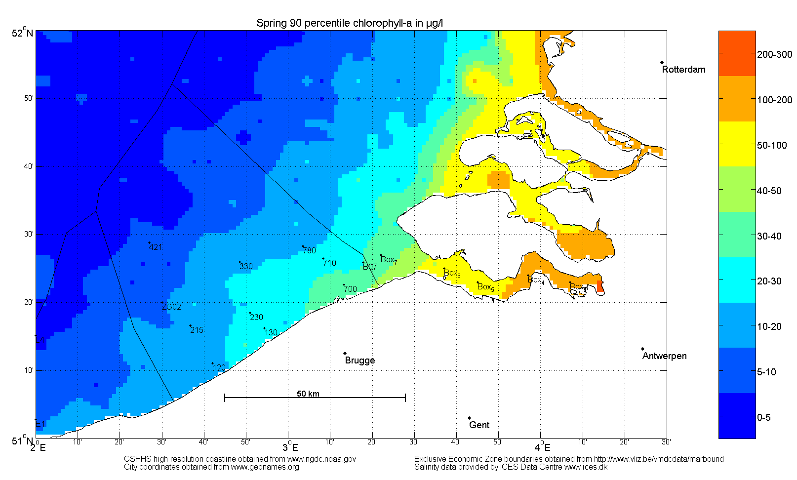
The values have been obtained by two-dimensional interpolation of salinity data provided by the ICES Oceanographic Database [2] and a "mixing diagram" for the dependency between the winter DIN levels and practical salinity for the Belgian Coastal Waters under pristine and actual conditions, as reported by the Belgian OSPAR workgroup conditions [3] during 2000-2005, and another linear relationship between the winter DIN and spring chlorophyll-a content [3]. The interpolation is based on the 2D interpolation algorithm by John d'Errico [4]. The critical assessment (elevated) level is assumed to be 50 % above the pristine level (OSPAR criterion). A nitrogen balance model [5] is used for the Scheldt river basin, which runs through France, Belgium and the Netherlands ending in the Westerscheldt estuary. The model is used to determine the impact of different measures to reduce the nitrogen outflow to coastal waters, such as reduction of the fertilizer use and cattle stock size. Finally, these scenarios are combined with the results of the 2D interpolation to derive the pattern of water quality parameters related to eutrophication such as the P90 (90^th percentile) value of chlorophyll-a.

Twelve scenarios are available on the Web Application Server:

1. Business-as-usual scenario: no action taken, result is reduction of 2.2 % in total nitrogen load by 2050 compared to the year 2010.
2. Gradual decrease of fertilizer use to 50 % of the initial value by 2040 (23 % reduction nitrogen load by 2050).
3. Buffer strips along receiving streams are considered a potentially useful means to achieve nutrient retention (Vermaat et al., 2012). Gradual increase in the use of buffer strips along river streams bordering agricultural land with a maximum width in the range of 10-50 m in the year 2040 (depending on the provence). This leads to a 18.5 % reduction in the nitrogen load by 2050.
4. Gradual decrease of the cattle stock size with 50 % by the year 2040 (24.6 % reduction in the nitrogen load by 2050).
5. Gradual improvement in the efficiency of waste-water treatment plants with 40 % by the year 2040 (13.6 % reduction in the nitrogen load by 2050).
6. Gradual reduction in the industrial effluents of nitrogen to 0 % by 2040 (resulting in 12.7 % reduction in the nitrogen load by 2050).
7. Gradual reduction in the effluents from households which are not connected to the waste-water treatment system to 0 % by 2040 (26.5 % reduction in the nitrogen load by 2050).
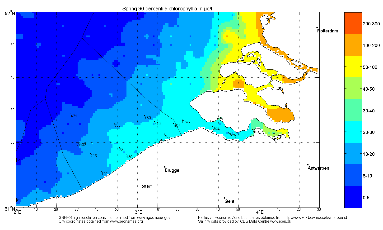
8. All management alternatives B-G combined (78.3 % reduction in the nitrogen load by 2050).
9. Business-as-usual with KNMI climate change scenario G [6] - unchanged circulation pattern with 1 degree celsius increase in temperature. KNMI 2006 Climate Change Scenarios see www.knmi.nl (results in 2 % reduction nitrogen load).
10. Business-as-usual with KNMI climate change scenario W+ [6] - changed circulation pattern with 2 degrees celsius increase in temperature. KNMI 2006 Climate Change Scenarios see www.knmi.nl (results in 5.4 % reduction nitrogen load).
11. In addition two other scenarios are available: one for the pristine conditions (based on the mixing diagram reported in OSPAR (2008)), and one for the critical OSPAR threshold (50 % above the pristine level).

As an example we compare the P90 value of chlorophyll-a for scenarios A (business-as-usual) and H (all measures combined) for the Belgian coastal waters:

References:

1. Eutrophication Status of the OSPAR Maritime Area, Second OSPAR Integrated Report, Table 4.6. Eutrophication Series. OSPAR Commission, 2008. www.ospar.org.
2. ICES, 2012. International Council for the Exploration of the Sea Oceanographic Database, 2012. ICES, Copenhagen. www.ices.dk.
3. OSPAR, 2008. Report on the second application of the OSPAR Comprehensive Procedure to the Belgian Marine Waters. Report by Belgium. Federal Public Service Health, Food Chain Safety and Environment, 70 pages, 2008. www.ospar.org.
4. John d'Errico (2006). www.mathworks.com/matlabcentral/fileexchange/4551
5. Vermaat, J.E., Broekx, S., Van Eck, B., Engelen, G., Hellmann, F., De Kok, J.L., Van der Kwast, H., Maes, J., Salomons, W. and Van Deursen, W., 2012. Nitrogen source apportionment for the catchment, estuary and adjacent coastal waters of the Scheldt, Special Issue - A Systems Approach for Sustainable Development in Coastal Zones, Ecology and Society 17 (2): 30.
6. Royal Netherlands Meteorological Institute (KNMI), Climate in the 21st Century: 4 scenarios for the Netherlands, 2006. www.knmi.nl/klimaatscenarios/knmi_nl_Ir.pdf.